The complexity of calculus is only superficial

Calculus provided relief from the two-thousand-year decline in mathematics that proceeded the death of Archimedes.¹ With its tools to analyze motion, change, and infinite series, calculus was a novel interpretation of reality and, to many, impossible to understand. Probably more often than not, students have gone into studying this subject with rumors of its difficulty floating in their mind, and, accordingly, they find it intractable. After years of calculus study, however, I find this widespread impression to be false.

I cannot generalize my claim over the entirety of calculus just yet, considering I am still only on Calc II, but I thoroughly believe that what I have to say is applicable to all students who are new to the subject.

Background

Since the 10th grade, I have been rigorously studying calculus. This was an unconventional place to begin since most students start learning the subject as a junior, senior, or college student (if they learn it at all, that is). Despite the breach in etiquette, however, my understanding flourished.

Having this reasonably smooth journey into calculus, I never quite understood people’s hesitation with the subject. Even stranger, I have heard some describe the transition of algebra to calculus as orders of magnitude more difficult than the transition from arithmetic to algebra. For me, though, I had more difficulty with algebra in 6th grade than calculus in 10th.

Understanding that I do not even remotely qualify as a genius, why was it that my 14-year-old self had no trouble with calculus, but a multitude of older students struggle with it.

The Proliferated Rumor

One reason that was alluded to earlier is culture. There is no shortage of people who will tell you that calculus is complicated, that it is not intuitive, that it is next-to-impossible to understand. It is probably more difficult to find someone to say otherwise.

Let me make my stance clear: I am not arguing that calculus is immediately accessible; I am arguing that the subject is fundamentally simple and not far from intuition. If this was not the case, humans probably never would have discovered it!

The other problem, of course, is having a teacher who is not enthusiastic about it themselves or perhaps doesn’t understand it. This is far too common. With a bad teacher, the student cannot parse the subject and will be left with the impression that the difficulty is an inherent property of the subject, instead of just the environment he or she learned it in.

My philosophy, which I think applies to nearly everything, is that complex things are usually just a lot of simple things densely packed together. It is your job as a student to unpack it.

If the reader is just starting calculus, I recommend skipping to the General Advice section below. The next two sections will be explanations of concepts commonly considered to be hard, but are actually straightforward.

Delta-Epsilon Proofs

Of all the concepts discussed in Calc I, the concept considered hardest is the $\delta$ – $\varepsilon$ (delta-epsilon) proof; yet, all the proofs you have to do will follow the same procedure. Here, I will attempt to explain the simplicity of $\delta$ – $\varepsilon$ proofs via an intuitive explanation and examples.

What is it?

Everything in math needs to be shown that it logically follows from the basic axioms of math. We demonstrate this via mathematical proofs. The $\delta$ – $\varepsilon$ proof is the proof of a limit.

Definition

The definition of a limit is as follows (where $a$ and $L$ are real numbers).

Let $f(x)$ be defined for all $x$ in some open interval containing the number $a$ , with the possible exception that $f(x)$ may or may not be defined at $a$ . We will write

$\lim_{x \to a} f(x) = L$

if given any number $\varepsilon > 0$ , we can find a number $\delta > 0$ such that $f(x)$ satisfies

$|f(x) - L| < \varepsilon$ whenever $x$ satisfies $0 < |x - a| < \delta$

Explanation

To the novice, this can be unsightly; however, this is actually quite simple.

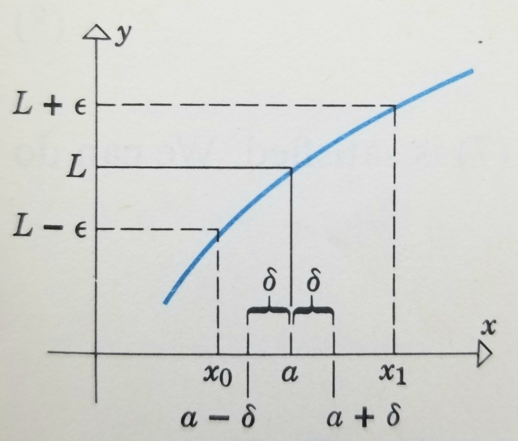
Limits are trying to find the value that $f(x)$ is converging to as $x$ is converging to $a$ . They are thus only concerned with the function behavior when $x$ is near but different from $a$ . This is why the definition is constructed with ranges around $a$ and $L$ .

In simple terms, the definition states that no matter how small some number $\delta$ is, eventually, as $x$ gets really close to $a$ , the distance between $x$ and $a$ (i.e. $|x - a|$ ) will be less than $\delta$ . Thus, $\delta$ could be equal to $10^{-100000}$ units, and, eventually, as $x$ approaches $a$ , the distance between them will become less than $10^{-100000}$ . Further, the limit definition states that as $x$ is approaching asymptotically close to $a$ , the corresponding $f(x)$ is getting closer to $L$ (see figure below — the $\delta$ range around $a$ is a subset of $(x_0, a) \cup (a, x_1)$ and is not shown). Indeed, as $x$ gets closer and closer to $a$ , $f(x)$ gets closer and closer to $L$ such that no matter how small some positive number $\varepsilon$ is, eventually the distance between $f(x)$ and $L$ will be smaller than it.

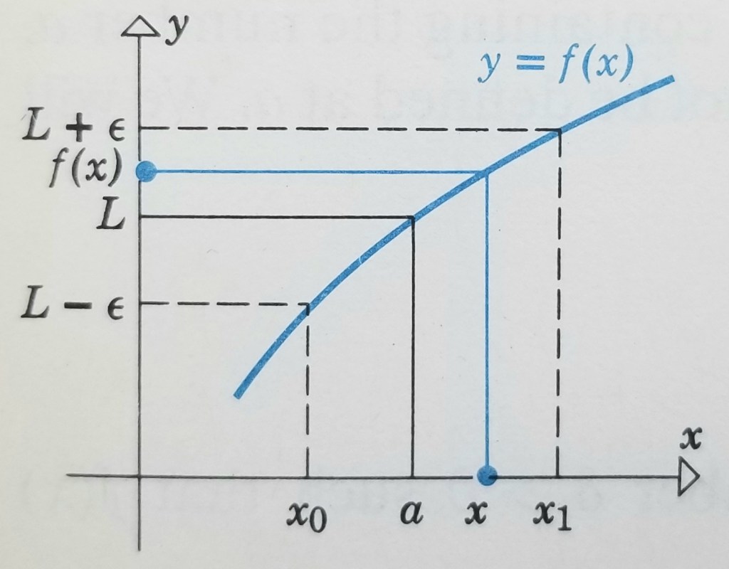
Below illustrates the $\delta$ range. As you can see, whenever the distance between $x$ and $a$ is less than $\delta$ , the distance between $f(x)$ and $L$ is less than $\varepsilon$ . In other words, when $x$ is in the $\delta$ range, $f(x)$ is in the $\varepsilon$ range.

Why is the $\boldsymbol{x}$ condition greater than zero, but the $\boldsymbol{f(x)}$ condition not?

The $f(x)$ condition is not greater than zero because $f(x)$ could assume the value $L$ at some point as $x$ approaches $a$ . In most diagrams, you will usually only see $f(a) = L$ (as for above), but this is not always true. For example, the constant function, $f(x) = L$ , will assume the value of $L$ as $x$ approaches $a$ . If we decided to stipulate that the distance between $f(x)$ and $L$ has to be greater than zero, we would not have a very good definition because we would not be able to take the limit of constant functions.

The $x$ condition is greater than zero because $x$ is not allowed to equal $a$ . A limit is supposed to tell you what value a function seems to be approaching. It thus only looks at the function values of $x$ around $a$ . Considering the value when $x$ equals $a$ would defeat the purpose of the limit.

What the problems consist of and how to solve them

Delta-epsilon proof problems that are given to the already struggling student generally look like this: “Prove [insert some limit here].”

To solve these, you will have to show that the given limit statement obeys the limit definition, viz. for every $\varepsilon$ satisfying the $f(x)$ condition there exists $\delta$ satisfying the $x$ condition. In order to show this, you will have to plug in the given $f(x)$ and $L$ into the $f(x)$ condition and plug in the given $a$ into the $x$ condition. After this, you have to find a formula that connects $\delta$ and $\varepsilon$ . Now, via the formula, whatever $\varepsilon$ you choose, there is automatically a corresponding $\delta$ . This satisfies the definition (read the definition again if what I just said is confusing).

That’s literally all. You just have to find a formula that connects $\varepsilon$ and $\delta$ .

The trickiest part, however, is going about finding the formula. To do so, you will have to algebraically manipulate the $f(x)$ condition until it looks like the $x$ condition. When you reduce the $f(x)$ condition with its restriction down to the $x$ condition, you will get a restriction on the $x$ condition. Earlier, we represented the $x$ condition’s restriction by the Greek letter $\delta$ , since we didn’t know the restriction at the time. Now, from this reduction, we know the restriction. We can then write $\delta$ is equal to this restriction, which is in terms of epsilon. That’s the formula.

This will make more sense with some…

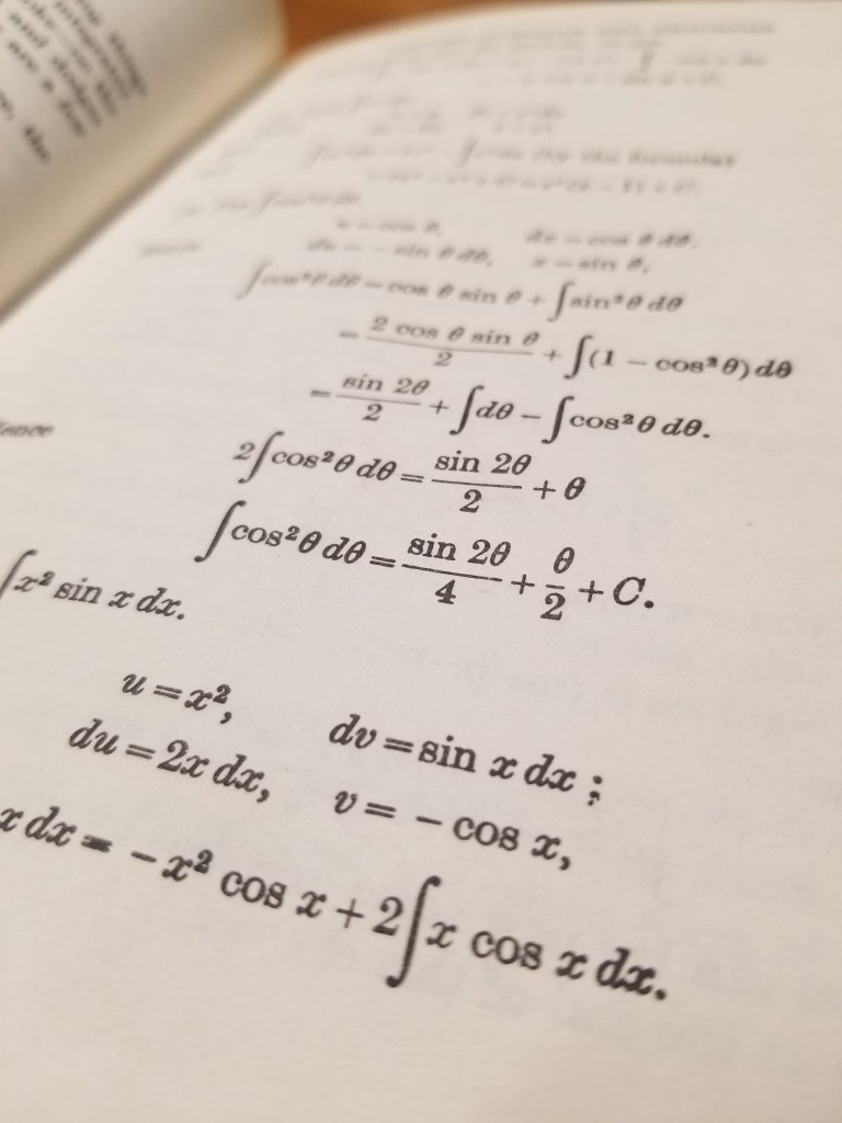
Examples

Prove $\lim_{x \to 2} (3x - 5) = 1$

Soln. We must show that given any positive number $\varepsilon$ , we can find a positive number $\delta$ such that $f(x) = 3x - 5$ satisfies

$|(3x - 5) - 1| < \varepsilon$ (i)

whenever $x$ satisfies

$0 < |x - 2| < \delta$ (ii)

As stated earlier, to find the formula for $\delta$ , we must manipulate the $f(x)$ condition until it looks like the $x$ condition. We can rewrite (i) as

$|3x - 6| = 3|x - 2| < \varepsilon$

$|x - 2| < \frac{\varepsilon}{3}$ (iii)

Remember: We have to choose a value for $\delta$ such that whenever we know $\varepsilon$ , we know $\delta$ . What (iii) is telling us is that the $x$ condition is less than $\frac{\varepsilon}{3}$ . Earlier, in (ii), we defined the boundary of the $x$ condition to be $\delta$ . This $\delta$ was just a placeholder for a value we didn’t yet know. Now, we have the boundary for the $x$ condition as $\frac{\varepsilon}{3}$ . Thus,

$\delta = \frac{\varepsilon}{3}$

We have just shown that for a given $\varepsilon$ satisfying (i), there exists a $\delta$ satisfying (ii). In other words, the conditions of the limit definition are satisfied. Therefore, the limit is true.

Done! It has been proven.

To analyze what we just did: We assumed that for any $\varepsilon$ satisfying the $f(x)$ condition there is a $\delta$ satisfying the $x$ condition. We didn’t know whether this was true, but we assumed it was and showed that this assumption was, in fact, correct. We showed this by using some algebra to reduce the $f(x)$ condition down to the $x$ condition. From this, we found the restriction of the $x$ condition in terms of $\varepsilon$ . This condition is such that, when $x$ satisfies it, the distance between $f(x)$ and $L$ is less than $\varepsilon$ . We then deduced that $\delta$ must be equal to this restriction. In this way, we satisfy the definition that for every $\varepsilon$ , there is a corresponding $\delta$ .

Limit proofs of linear functions are about as easy as $\delta$ – $\varepsilon$ proofs get. Any further and you have to be more creative with the algebraic manipulations of the $f(x)$ condition. However, it is still the same underlying principle; i.e. find $\delta$ in terms of $\varepsilon$ .

A bit harder of an example

Prove $\lim_{x \to a} x^2 = a^2$

Soln. This is more abstract than the last one, but our goal is still the same. Assume we are given an $\varepsilon > 0$ . Find that there is $\delta$ for every $\varepsilon$ such that

$|x^2 - a^2| < \varepsilon$ (i)

whenever

$0 < |x - a| < \delta$ (ii)

We need to manipulate the $f(x)$ condition so that it looks like the $x$ condition. This way we find the restriction on the $x$ condition. That restriction will be equal to our restriction placeholder, $\delta$ . Thus, we do as follows:

$|x^2 - a^2| = |x + a||x - a| < \varepsilon$

Okay, so we have our $|x - a|$ condition expressed here, which is good. However, we also have this other factor, $|x + a|$ . It’s fine to have factors that are constant, but this one varies with $x$ . The bad thing about this is we don’t really know its behavior. In general, there are cases where we can write $|f(x) - L|$ as $|g(x)||x - a|$ , where $|g(x)|$ is a non-constant function and $|x - a|$ is the $x$ condition. WE DON’T KNOW THE BEHAVIOR OF $|g(x)|$ !!! It could very well be that, as $x$ approaches $a$ , the value of $|g(x)|$ blows up to infinity. If that happens, it doesn’t matter that $|x - a|$ is getting smaller; $|g(x)|$ ruins any hope of $|g(x)||x - a| < \varepsilon$ . Therefore, we cannot isolate the $x$ condition. We must restrict (or bound) our non-constant factor’s value to be such that the product, $|x + a||x - a|$ , remains less than $\varepsilon$ . How do we do this? We constrain the value of $x$ to only a set range of values, wherein the value of $|x + a|$ is such that the product is less than $\varepsilon$ . The range of $x$ is determined by allowing $\delta$ to equal some value, say, $1$ :

Let $\delta = 1$ . Then,

$0 < |x - a| < 1 \implies -1 < x - a < 1 \implies a - 1 < x < 1 + a \implies |x| < |1 + a| \leq 1 + |a|$

The boundary value that $x$ has in order to satisfy $\delta = 1$ is $1 + a$ . Thus, the range of $|x + a|$ when $\delta$ equals 1 is

$|x + a| \leq |x| + |a| < 1 + |a| + |a| = 1 + 2|a|$

This is our boundary wherein the product $|x + a||x - a|$ is less than $\varepsilon$ :

$|x + a||x - a| < (1 + 2|a|) |x - a| < \varepsilon$

Now, we need a range of $|x - a|$ where $(1 + 2|a|) |x - a|$ is indeed less than $\varepsilon$ . Thus,

$|x - a| < \frac{\varepsilon}{1 + 2|a|}$

But, hold on. We had put $|x - a| < \delta$ . We put $\delta$ to represent the restriction we had yet to know. But now, we know the restriction for $|x - a|$ is $\frac{\varepsilon}{1 + 2|a|}$ . Thus,

$\delta = \frac{\varepsilon}{1 + 2|a|}$

With this, no matter what value of $\varepsilon$ we are given, we know the value of $\delta$ .

This value of $\delta$ satisfies the condition that $|x - a| < \frac{\varepsilon}{1 + 2|a|}$ (obviously), but we also need the condition of $|x - a| < 1$ to be satisfied. Otherwise, our non-constant factor wouldn't be bounded. (The following answer is seen to be valid from the observation that for any value of $\delta$ we choose, any value smaller than that would also work.)

Thus, for the value of $\delta$ we choose the minimum of $\frac{\varepsilon}{1 + 2|a|}$ and $1$ . This is denoted as

$\delta =$ $\min$ $\{$ 1 , $\frac{\varepsilon}{1 + 2|a|}$ $\}$

We interpret this result as “Whatever value is smaller, we make delta equal to that.” This way, (i) is satisfied whenever (ii) is satisfied.

Q.E.D.

N.B. The choice of $1$ as the value of $\delta$ was arbitrary. It could have been $3$ or $\frac{1}{4}$ just as well, but the standard choice is $1$ .

Harder example

Prove $\lim_{x \to \frac{1}{2}} \frac{1}{x} = 2$

Soln. We assume that for any given $\varepsilon > 0$ , we can find a $\delta > 0$ such that

$\left|\frac{1}{x} - 2\right| < \varepsilon$ (i)

whenever

$0 < \left| x - \frac{1}{2} \right| < \delta$ (ii)

We must manipulate the $f(x)$ condition to look like the $x$ condition, so that we can find the restriction on $|x - \frac{1}{2}|$ . This restriction will be equal to $\delta$ . Thus,

$\left|\frac{1}{x} - 2\right| = \left|\frac{2}{x}\right| \left| x - \frac{1}{2} \right| < \varepsilon$

We have rewritten (i) to have (ii) as a factor. But… oh no. Not again! We have a non-constant factor, $\left|\frac{2}{x}\right|$ . As I said before, we must bound this factor in order to assure ourselves that the product is less than $\varepsilon$ when $x$ approaches $\frac{1}{2}$ . To do so, we let $\delta = \frac{1}{4}$ ( $\delta$ can’t equal 1 because the value $\left|\frac{2}{x}\right|$ goes ad infinitum when it approaches $x = 0$ ), find the range of $x$ that satisfies such a restriction, and then find the boundary of the $\left|\frac{2}{x}\right|$ . This way, the product, $\left|\frac{2}{x}\right| \left| x - \frac{1}{2} \right|$ , remains less than $\varepsilon$ .

Let $\delta = \frac{1}{4}$ ,

$0 < \left| x - \frac{1}{2} \right| < \frac{1}{4} \implies -\frac{1}{4} < x - \frac{1}{2} < \frac{1}{4} \implies \frac{1}{4} < x < \frac{3}{4}$

The range of $x$ that obeys $\delta = \frac{1}{4}$ is $($ $\frac{1}{4}$ , $\frac{3}{4}$ $)$ . To obtain the boundary for $\left|\frac{2}{x}\right|$ , let us take the reciprocal of the inequality and multiply by 2:

$\frac{1}{4} < x < \frac{3}{4}$ $\implies$ $4 > \frac{1}{x} > \frac{4}{3}$ $\implies$ $8 > \frac{2}{x} > \frac{8}{3}$

Thus, $\left|\frac{2}{x}\right| < 8$ . This boundary is such that, when it is obeyed, the product, $\left|\frac{2}{x}\right| \left| x - \frac{1}{2} \right|$ , is less than $\varepsilon$ . It is then true that

$\left|\frac{2}{x}\right| \left| x - \frac{1}{2} \right| < 8 \left| x - \frac{1}{2} \right| < \varepsilon$

We need to choose a restriction of $\left| x - \frac{1}{2} \right|$ that allows this to be true. If $\left| x - \frac{1}{2} \right|$ remains less than $\frac{\varepsilon}{8}$ , the strict inequality is satisfied. Thus,

$\left|\frac{2}{x}\right| \left| x - \frac{1}{2} \right| < 8 \left| x - \frac{1}{2} \right| < 8 \left(\frac{\varepsilon}{8}\right) = \varepsilon$

But hold on… we made $|x - \frac{1}{2}| < \delta$ . That $\delta$ merely represented the restriction of the $x$ condition. Now, we have found the restriction of $|x - \frac{1}{2}|$ to be $\frac{\varepsilon}{8}$ . Thus,

$\delta = \frac{\varepsilon}{8}$

With this, no matter what value of $\varepsilon$ is given, we know the value of $\delta$ . That is to say, for every $\varepsilon > 0$ , there exists a $\delta > 0$ such that (i) and (ii) are satisfied. We need to include, however, our arbitrary value of $\delta = \frac{1}{4}$ , so that the non-constant factor remains bounded, which requires $\left| x - \frac{1}{2} \right| < \frac{1}{4}$ . We also need $\left| x - \frac{1}{2} \right| < \frac{\varepsilon}{8}$ . We pick whichever value is smallest. Thus,

$\delta = \min\left\{\frac{1}{4}, \frac{\varepsilon}{8}\right\}$

Q.E.D.

In conclusion of $\mathbf{\delta\text{-}\epsilon}$ proofs

For the delta-epsilon proof, the goal is to choose $\delta$ based on a given $\varepsilon$ so that $0 < |x - a| < \delta \implies |f(x) - L| < \varepsilon$ . The answer will be a formula for $\delta$ in terms of $\varepsilon$ . There are cases where this procedure is made difficult by a non-constant factor popping up during our reduction of $|f(x) - L|$ to $|x - a|$ . The goal, however, remains the same.

Optimization Problems

Problems concerned with finding the most optimal way to perform a task are called optimization problems.

It’s strange to learn that many people find these to be difficult, considering a large swath of optimization problems are simply finding the largest or smallest value of a function and determining where the value occurs. I personally love this part of calculus. It requires logic and a healthy amount of creativity.

What are you required to do?

For optimization problems, you will have a constraint that is used to isolate one variable and a formula/function to maximize or minimize. You thus do as follows: Using the constraint, express the function in terms of one independent variable. Find the range of values that the variable can equal such that the context of the problem is satisfied. Differentiate the function. Set the derivative equal to zero and find the value of the variable that leads to such a condition being true. You now have candidates for the maximum or minimum. Find which one is the relevant extremum.

Why do we set the derivative equal to zero?

Since we are trying to find the relative extrema of functions, we have to solve for points that have the properties of relative extrema. All points that are relative maxima or minima have derivatives of zero. In other words, the tangent line at a relative extremum is horizontal. We thus solve for points that have derivatives of zero and narrow down the candidates to the actual extremum.

Examples

With reference to the diagram below:

Find the dimension of a rectangle with perimeter 100ft whose area is as large as possible.

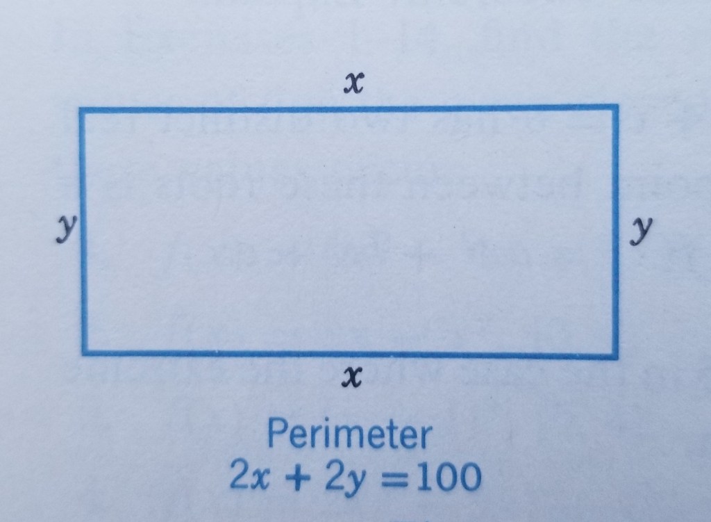
Soln. Let

$x = \text{length of rectangle}$

$y = \text{width of rectangle}$

$A = \text{area of rectangle}$

Then

$A = xy$

Since the perimeter of the rectangle is 100 ft, the variables $x$ and $y$ are related by the equation:

$2x + 2y = 100$

Notice, we are told to find the dimensions of the rectangle whose area is largest. We thus have to solve for the dimensions when the area is at a maximum. The formula $A = xy$ is the formula we must maximize, but we need it in terms of just one variable. To do this, we use our relation between $x$ and $y$ (this is the constraint I talked about earlier) to solve for one variable.

$2x + 2y = 100 \implies y = 50 - x$

Using substitution,

$A = x(50 - x) = 50x - x^2$

Because $x$ represents a length, it cannot be negative. Additionally, since the two sides of length $x$ cannot have a combined length exceeding the total perimeter of 100 ft, the variable must satisfy

$0 < x < 50$

It can’t equal $0$ because we’d then have a one-dimensional line with no area. It can’t equal $50$ because then $y$ would equal zero and that would once again just be a line. (Some opt to include those as endpoints, since they are mathematically possible. However, I am in the camp that believes humanity should not waste its time by considering practically impossible things.)

Differentiate $A$ :

$\frac{dA}{dx} = 50 - 2x$

Create the conditional statement of $\frac{dA}{dx} = 0$ (to find the relative extrema) and solve for values of $x$ that satisfy the condition.

$\frac{dA}{dx} = 50 - 2x = 0$

The solution is $x = 25$ . From the relation, $y = 25$ .

The rectangle of perimeter 100ft with greatest area is a square with sides of length 25ft.

A bit harder of an example

With reference to the diagram below:

An offshore oil well is located in the ocean at a point W, which is 5 mi from the closest shorepoint A on a straight shoreline. The oil is to be piped to a shorepoint B that is 8 mi from A by piping it on a straight line underwater from W to some shorepoint P between A and B and then on to B via a pipe along the shoreline. If the cost of laying pipe is $100,000 per mile underwater and $75,000 per mile over land, where should the point P be located to minimize the cost of laying the pipe?

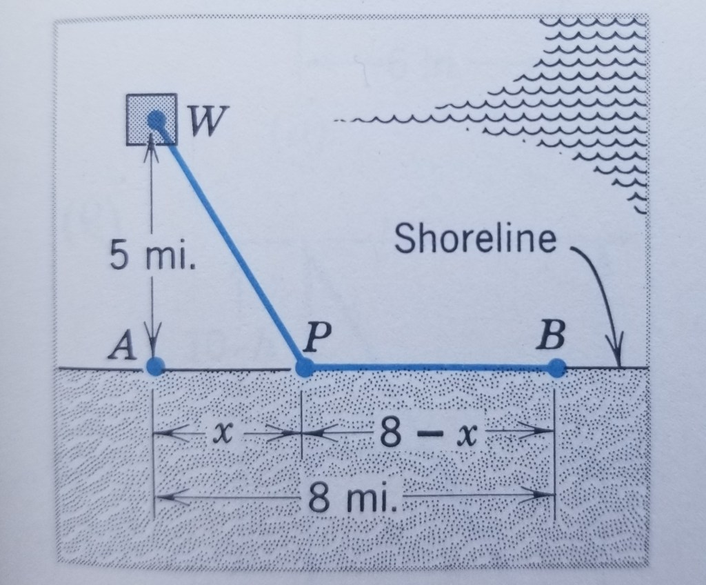
(Remark. The shortest distance between W and B would, indeed, be a straight line. Even though this uses the least amount of pipe, all of it is underwater, which would be expensive to lay. Similarly, a pipeline from W to A to B uses the least amount of expensive underwater pipe, but uses the greatest total amount of pipe. Thus, it is actually best to make a pipeline that goes from W to some point P between A and B and then go on to B. This would incur less total cost than by piping to either extreme location.)

Soln. Let

$x = \text{distance (in miles) between A and P}$

$C = \text{cost (in thousands of dollars) for the entire pipeline}$

We see from the diagram that the distance of pipe underwater from W to P is

$\sqrt{x^2 + 25} \text{ miles}$ (i)

We also see that the distance between the P and B is

$8 - x \text{ miles}$ (ii)

From (i) and (ii), the total cost $C$ (in thousands of dollars) for the pipeline is

$C = 100 \sqrt{x^2 + 25} + 75 (8 - x)$

Because the distance between A and B is 8 mi, the distance between A and P must satisfy

$0 \leq x \leq 8$

(We include the endpoints, since they are practically possible.) In this problem, we have no constraint, which is fine since the formula is already in terms of one variable. Differentiate $C$ :

$\frac{dC}{dx} = \frac{100x}{\sqrt{x^2 + 25}} - 75$

Equating $\frac{dC}{dx}$ to zero,

$\frac{100x}{\sqrt{x^2 + 25}} - 75 = 0$

$\frac{4x}{\sqrt{x^2 + 25}} - 3 = 0$

$4x = 3\sqrt{x^2 + 25}$

$16x^2 = 9(x^2 + 25)$

$7x^2 = 225$

$x = \pm \frac{15}{\sqrt{7}}$

The number $-\frac{15}{\sqrt{7}}$ is not within our range, leading $\frac{15}{\sqrt{7}}$ being the only stationary point. The minimum thus occurs at one of the following points:

$x = 0, \quad x = \frac{15}{\sqrt{7}}, \quad x = 8$

Plugging these values into the cost formula yields

When $x = 0, \quad C = 1100$

When $x = \frac{15}{\sqrt{7}}, \quad C \approx 930.719$

When $x = 8, \quad C \approx 943.398$

We need the value of $x$ such that $C$ is a minimum. The answer is therefore $x = \frac{15}{\sqrt{7}}$ .

The distance of P, the point onshore where we pipe the oil to, must be $\frac{15}{\sqrt{7}}$ mi away from A in order for the cost to be a minimum.

A harder example

With reference to the diagram below:

Find a point on the curve $y = x^2$ that is closest to the point $(18, 0)$

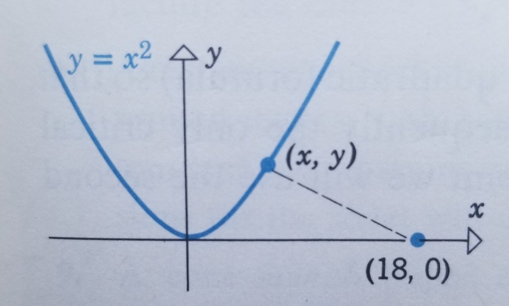
Soln. The distance $L$ between $(18, 0)$ and an arbitrary point $(x, y)$ on the curve $y = x^2$ is given by the Euclidean distance formula:

$L = \sqrt{(x - 18)^2 + (y - 0)^2}$

Since $(x, y)$ lies on the curve, $x$ and $y$ must satisfy $y = x^2$ . Thus,

$L = \sqrt{(x - 18)^2 + x^4}$ (formula to minimize)

Because there are no restrictions on $x$ , the problem reduces to finding a value of $x$ in $(-\infty, +\infty)$ for which $L$ is a minimum, provided such a value exists.

I am going to use a helpful math trick that is based on the following fact: The maxima and minima of a function occur at the same points as the square of that function. Thus, the minimum value of $L$ and the minimum value of

$S = L^2 = (x - 18)^2 + x^4$

occur at the same $x$ value.

Differentiate $S$ :

$\frac{dS}{dx} = 2(x - 18) + 4x^3 = 4x^3 + 2x - 36$

Equate to zero:

$4x^3 + 2x - 36 = 0 \implies 2x^3 + x - 18 = 0$

The only real solution to this conditional statement is $x = 2$ . The second derivative test yields a positive result when $x = 2$ is plugged in. Thus, the point on $y = x^2$ that is closest to the point $(18, 0)$ is

$(x, y) = (x, x^2) = (2, 4)$

In summary of optimization problems

These types of problems almost always follow the same procedure.

Step 1: Label the quantities relevant to the problem.

Step 2: Find the formula to be maximized or minimized.

Step 3: Using the conditions stated in the problem to eliminate variables, express the quantity to be maximized or minimized as a function of one variable.

Step 4: Find the interval of possible values for this variable from the physical restrictions in the problem.

Step 5: The rest is mechanical. Differentiate the function. Equate to zero. Find the values of the variable that satisfy that condition. Determine which value is correct via the range and whether it is the appropriate type of extremum.

General Advice

This subject is not as hard as you have been led to believe. Certainly, it is hard to intuit at first, but with many hours of focused study, it will start to become clearer. People who experience zero friction with intellectually-taxing studies do not exist; those you think do simply work hard and often.

For any student just beginning this wonderful yet difficult subject, the following list might provide good advice:

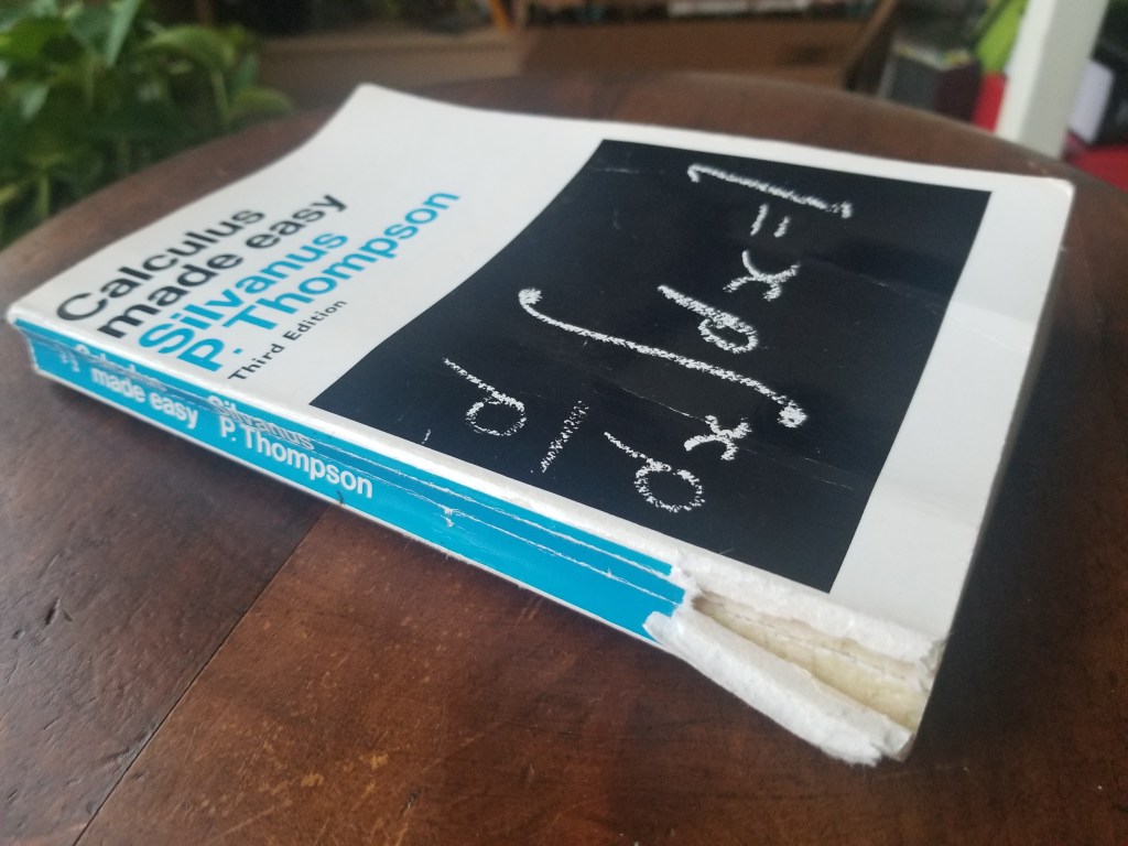
Read respected books – One reason why my 14-year-old self was able to understand calculus quickly was the literature I used. If you are struggling with this subject, I highly recommend Thompson’s Calculus made easy. The book explains everything extremely well and acknowledges its quasi-complexity. It is not, however, a formal math book, and you should try to get through it as quickly as understanding permits so that more formal textbooks can be tackled.

Don’t be scared by weird-looking symbols – There are a lot of strange ones in calc; however, they all have precise meanings and will be comforting to see once they are learned.

Master algebra and trig – Calculus definitely requires a firm understanding of algebra and trigonometry, so be sure to get sufficiently good at those. For me personally, however, I started with only a basic understanding of trig and was able to learn calc efficiently. If I ran across any trigonometry concept I didn’t recognize, I would divert time to learn it.

Ask questions – It is more productive to be confused and know specifically why than to just be confused. Try to reduce your confusion to specific questions that can actually be answered and then seek answers either by thinking on your own or by consulting an external source. (If you don’t understand parts of this blog, apply this method.)

Don’t lose the plot – The simplicity will beget complexity. You cannot forget that, at its core, it is made up of the same simple things.

In summary, just work hard. There is no substitute for work, and a skill is impossible to obtain without practicing it frequently. You will often hear mathematicians speak of the beauty of their subject. This probably sounds strange to the layperson, but rigorous study of calculus will make that claim less unreasonable. You will start to see the underlying simplicity of it all and realize why it has to be the way that it is.

And after you have finished the material and are comfortable with the subject, be proud to have such a well-thumbed book on your shelf. It is a very satisfying sign of progress.

This is an oversimplification of those 2000 years. The decline was primarily in the Western world. Most of the progress made in that time was by China, India, and the Islamic world. Also, the decline is considered to have actually ended about 100 years before the discovery of calculus, with Copernicus’ De Revolutionibus. ↩︎

Background

The Proliferated Rumor

Delta-Epsilon Proofs

Optimization Problems

General Advice

Share this:

Related